3D vector field and image across time

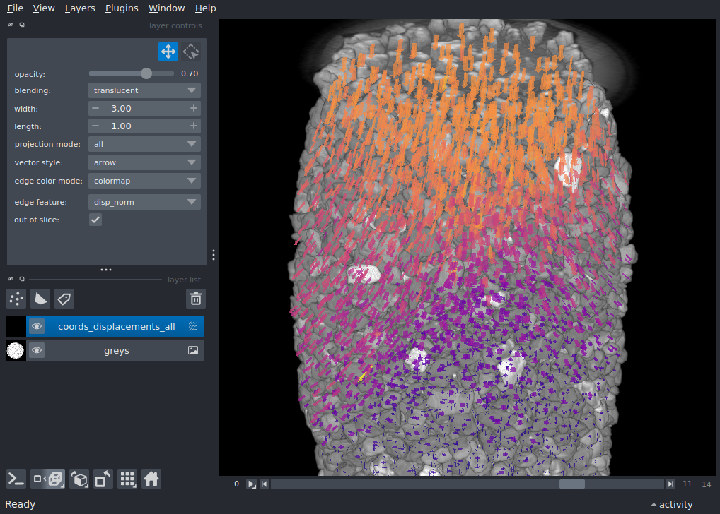
This example is from a mechanical test on a granular material, where multiple 3D volume have been acquired using x-ray tomography during axial loading. We have used [spam](https://www.spam-project.dev/) to label individual particles (with watershed and some tidying up manually), and these particles are tracked through time with 3D “discrete” volume correlation incrementally: t0 → t1 and then t1 → t2. Although we’re also measuring rotations (and strains), but here we’re interested to visualise the displacement field on top of the image to spot tracking errors.

Tags: visualization-nD

import numpy as np
import pooch
import tifffile

import napari

Input data

Input data are therefore:

• A series of 3D greyscale images

• A series of measured transformations between subsequent pairs of images

• We also have consistent labels through time which could also be visualised but are not here

Let’s download it!

grey_files = sorted(pooch.retrieve(
    "doi:10.5281/zenodo.17668709/grey.zip",
    known_hash="md5:760be2bad68366872111410776563760",
    processor=pooch.Unzip(),
    progressbar=True
))

# Load individual 3D images as a 4D with a list comprehension, skipping last one
# result is a T, Z, Y, X 16-bit array
greys = np.array([tifffile.imread(grey_file) for grey_file in grey_files[0:-1]])

# load incremental TSV tracking files from spam-ddic, [::2] is to skip VTK files also in folder
tracking_files = sorted(pooch.retrieve(
    "doi:10.5281/zenodo.17668709/ddic.zip",
    known_hash="md5:2d7c6a052f53b4a827ff4e4585644fac",
    processor=pooch.Unzip(),
    progressbar=True
))[::2]

Downloading...
From (original): https://drive.google.com/uc?id=1UZEoOtHMMeJMXVoWr6IZraZnvQe8ExNJ
From (redirected): https://drive.google.com/uc?id=1UZEoOtHMMeJMXVoWr6IZraZnvQe8ExNJ&confirm=t&uuid=a9b67583-9bbf-4cc3-abce-ffb3b5b3d0d4
To: /home/runner/work/docs/docs/.cache/pooch/tmp6o435rs7

  0%|          | 0.00/549M [00:00<?, ?B/s]
  1%|          | 6.82M/549M [00:00<00:19, 27.3MB/s]
  2%|▏         | 13.1M/549M [00:00<00:13, 39.5MB/s]
  3%|▎         | 17.8M/549M [00:00<00:14, 36.2MB/s]
  4%|▍         | 22.0M/549M [00:00<00:18, 28.7MB/s]
  5%|▌         | 29.9M/549M [00:00<00:14, 34.7MB/s]
  6%|▋         | 35.7M/549M [00:00<00:12, 39.8MB/s]
  7%|▋         | 40.4M/549M [00:01<00:14, 35.9MB/s]
  9%|▊         | 46.7M/549M [00:01<00:13, 36.6MB/s]
 10%|█         | 55.1M/549M [00:01<00:18, 26.4MB/s]
 12%|█▏        | 65.5M/549M [00:01<00:14, 33.3MB/s]
 14%|█▍        | 76.0M/549M [00:02<00:12, 38.6MB/s]
 15%|█▌        | 84.9M/549M [00:02<00:09, 46.9MB/s]
 17%|█▋        | 90.7M/549M [00:02<00:10, 43.5MB/s]
 18%|█▊        | 97.0M/549M [00:02<00:10, 44.5MB/s]
 20%|█▉        | 107M/549M [00:02<00:09, 47.4MB/s]
 21%|██        | 113M/549M [00:02<00:09, 48.2MB/s]
 22%|██▏       | 118M/549M [00:03<00:09, 44.9MB/s]
 24%|██▎       | 129M/549M [00:03<00:06, 60.3MB/s]
 25%|██▍       | 136M/549M [00:03<00:06, 59.6MB/s]
 26%|██▋       | 145M/549M [00:03<00:06, 59.8MB/s]
 28%|██▊       | 152M/549M [00:03<00:06, 57.0MB/s]
 29%|██▉       | 158M/549M [00:03<00:07, 52.0MB/s]
 30%|███       | 167M/549M [00:03<00:06, 60.4MB/s]
 32%|███▏      | 175M/549M [00:03<00:06, 55.2MB/s]
 33%|███▎      | 182M/549M [00:04<00:06, 59.1MB/s]
 35%|███▍      | 191M/549M [00:04<00:06, 58.0MB/s]
 36%|███▋      | 200M/549M [00:04<00:06, 52.0MB/s]
 38%|███▊      | 211M/549M [00:04<00:05, 64.0MB/s]
 40%|███▉      | 218M/549M [00:04<00:05, 60.3MB/s]
 42%|████▏     | 230M/549M [00:04<00:04, 73.8MB/s]
 43%|████▎     | 239M/549M [00:05<00:06, 49.9MB/s]
 45%|████▍     | 245M/549M [00:05<00:05, 51.8MB/s]
 46%|████▌     | 252M/549M [00:05<00:06, 49.2MB/s]
 47%|████▋     | 260M/549M [00:05<00:05, 54.8MB/s]
 49%|████▊     | 267M/549M [00:05<00:04, 57.5MB/s]
 50%|████▉     | 274M/549M [00:05<00:04, 55.9MB/s]
 51%|█████     | 281M/549M [00:05<00:04, 59.3MB/s]
 52%|█████▏    | 287M/549M [00:05<00:04, 59.0MB/s]
 54%|█████▍    | 298M/549M [00:05<00:03, 72.1MB/s]
 56%|█████▌    | 306M/549M [00:06<00:04, 53.3MB/s]
 58%|█████▊    | 317M/549M [00:06<00:03, 58.7MB/s]
 59%|█████▉    | 324M/549M [00:06<00:04, 52.4MB/s]
 61%|██████    | 332M/549M [00:06<00:03, 56.9MB/s]
 62%|██████▏   | 340M/549M [00:06<00:03, 60.4MB/s]
 63%|██████▎   | 347M/549M [00:06<00:03, 59.3MB/s]
 65%|██████▍   | 355M/549M [00:07<00:03, 59.7MB/s]
 66%|██████▌   | 361M/549M [00:07<00:03, 58.8MB/s]
 68%|██████▊   | 373M/549M [00:07<00:02, 71.7MB/s]
 69%|██████▉   | 381M/549M [00:07<00:02, 64.5MB/s]
 71%|███████   | 391M/549M [00:07<00:02, 69.2MB/s]
 73%|███████▎  | 398M/549M [00:07<00:02, 69.5MB/s]
 74%|███████▍  | 405M/549M [00:07<00:02, 69.8MB/s]
 76%|███████▌  | 417M/549M [00:07<00:01, 81.5MB/s]
 78%|███████▊  | 425M/549M [00:07<00:01, 71.5MB/s]
 79%|███████▉  | 435M/549M [00:08<00:01, 72.0MB/s]
 81%|████████▏ | 447M/549M [00:08<00:01, 84.3MB/s]
 83%|████████▎ | 456M/549M [00:08<00:01, 68.9MB/s]
 85%|████████▌ | 467M/549M [00:08<00:01, 78.5MB/s]
 87%|████████▋ | 476M/549M [00:08<00:00, 73.4MB/s]
 89%|████████▊ | 487M/549M [00:08<00:00, 81.4MB/s]
 90%|█████████ | 495M/549M [00:08<00:00, 74.5MB/s]
 92%|█████████▏| 506M/549M [00:09<00:00, 67.5MB/s]
 94%|█████████▍| 515M/549M [00:09<00:00, 71.6MB/s]
 95%|█████████▌| 523M/549M [00:09<00:00, 66.2MB/s]
 97%|█████████▋| 530M/549M [00:09<00:00, 61.0MB/s]
 99%|█████████▉| 544M/549M [00:09<00:00, 77.6MB/s]
100%|██████████| 549M/549M [00:09<00:00, 56.5MB/s]
Downloading...
From: https://drive.google.com/uc?id=1-AAkBUXykxXG3Ve20jPk43co-m3f9ZWB
To: /home/runner/work/docs/docs/.cache/pooch/tmpvurwurzq

  0%|          | 0.00/6.72M [00:00<?, ?B/s]
 55%|█████▍    | 3.67M/6.72M [00:00<00:00, 31.7MB/s]
100%|██████████| 6.72M/6.72M [00:00<00:00, 45.0MB/s]

Collect data together for napari

We will loop through all the images in order to prepare the necessary data structure for napari

These variables are going to contain coordinates, displacements and lengths (for colouring vectors) for all timesteps

coords_all = []
disps_all = []
lengths_all = []

for t, tracking_file in enumerate(tracking_files):
    # load the indicator for convergence
    returnStatus = np.genfromtxt(tracking_file, skip_header=1, usecols=(19))

    # Load coords and displacements, keeping only converged results (returnStatus==2)
    coords = np.genfromtxt(tracking_file, skip_header=1, usecols=(1,2,3))[returnStatus==2]
    disps = np.genfromtxt(tracking_file, skip_header=1, usecols=(4,5,6))[returnStatus==2]

    # Compute lengths in order to colour vectors
    lengths = np.linalg.norm(disps, axis=1)

    # Prepend an extra dimension to coordinates to place them in time, and fill it with the incremental t
    coords = np.hstack([np.ones((coords.shape[0],1))*t, coords])
    # Preprend zeros to the displacements (the "end" of the vector), since they do not displace through time
    disps = np.hstack([np.zeros((disps.shape[0],1)), disps])

    # Add to lists
    coords_all.append(coords)
    disps_all.append(disps)
    lengths_all.append(lengths)

# Concatenate into arrays
coords_all = np.concatenate(coords_all)
disps_all = np.concatenate(disps_all)
lengths_all = np.concatenate(lengths_all)
# Stack this into an array of size N (individual points) x 2 (vector start and length) x 4 (tzyx)
coords_displacements_all = np.stack([coords_all, disps_all], axis=1)

viewer = napari.Viewer(ndisplay=3)

viewer.add_image(
    greys,
    contrast_limits=[15000, 50000],
    rendering="attenuated_mip",
    attenuation=0.333
)

viewer.add_vectors(
  coords_displacements_all,
  vector_style='arrow',
  length=1,
  properties={'disp_norm': lengths_all},
  edge_colormap='plasma',
  edge_width=3,
  out_of_slice_display=True,
)

viewer.camera.angles = (2,-11,-23.5)
viewer.camera.orientation = ('away','up','right')
viewer.dims.current_step = (11,199, 124, 124)


if __name__ == '__main__':
    napari.run()