Visualizing optical flow in napari

Adapted from the scikit-image gallery [1].

In napari, we can show the flowing vortex as an additional dimension in the image, visible by moving the slider.

Tags: visualization-advanced, layers

[1]

https://scikit-image.org/docs/stable/auto_examples/registration/plot_opticalflow.html

import numpy as np
from skimage.data import vortex
from skimage.registration import optical_flow_ilk

import napari

First, we load the vortex image as a 3D array. (time, row, column)

vortex_im = np.asarray(vortex())

We compute the optical flow using scikit-image. (Note: as of scikit-image 0.21, there seems to be a transposition of the image in the output, which we account for later.)

u, v = optical_flow_ilk(vortex_im[0], vortex_im[1], radius=15)

Compute the flow magnitude, for visualization.

magnitude = np.sqrt(u ** 2 + v ** 2)

We subsample the vector field to display it — it’s too messy otherwise! And we transpose the rows/columns axes to match the current scikit-image output.

nvec = 21
nr, nc = magnitude.shape
step = max(nr//nvec, nc//nvec)
offset = step // 2
usub = u[offset::step, offset::step]
vsub = v[offset::step, offset::step]

vectors_field = np.transpose(  # transpose required — skimage bug?
        np.stack([usub, vsub], axis=-1),
        (1, 0, 2),
        )

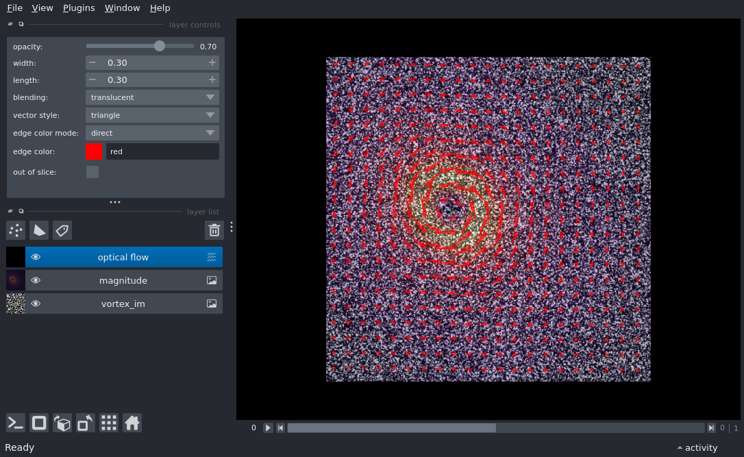
Finally, we create a viewer, and add the vortex frames, the flow magnitude, and the vector field.

viewer, vortex_layer = napari.imshow(vortex_im)
mag_layer = viewer.add_image(magnitude, colormap='magma', opacity=0.3)
flow_layer = viewer.add_vectors(
        vectors_field,
        name='optical flow',
        scale=[step, step],
        translate=[offset, offset],
        edge_width=0.3,
        length=0.3,
        )

if __name__ == '__main__':
    napari.run()