Using Dask and napari to process & view large datasets#
Often in microscopy, multidimensional data is acquired and written to disk in many small files, each of which contain a subset of one or more dimensions from the complete dataset. For example, in a 5-dimensional experiment (e.g. 3D z-stacks acquired for multiple channels at various moments over time), each file on disk might be a 3D TIFF stack from a single channel at a single timepoint. Data may also be stored in some proprietary format. As the size of the dataset grows, viewing arbitrary slices (in time, channel, z) of these datasets can become cumbersome.
Chunked file formats exist (such as hdf5 and zarr) that store data in a way that makes it easier to retrieve arbitrary subsets of the dataset, but they require either data duplication, or “committing” to a new file standard.
Note
This tutorial is not meant to promote a folder of TIFFs as a “good way” to store large datasets on disk; but it is
undoubtedly a common scenario in microscopy. Chunked formats such as hdf5 or zarr are superior in many ways, but
they do require the user to either duplicate their data or go “all in” and delete the original data after conversion.
And while napari can easily handle something like a zarr store, it can be a bit more limiting inasmuch as it
requires programs that are capable of viewing it (i.e. you can’t necessarily just drag it into Fiji …)
The first part of this tutorial demonstrates how to use Dask
and dask.delayed
(or dask_image) to feed napari image data “lazily”:
that is, the specific image file corresponding to the requested timepoint/channel
is only read from disk at the moment it is required
(based on the current position of the dimension sliders in napari).
Additionally, we will see that any function that takes a filepath
and returns a numpy array can be used to lazily read image data.
This can be useful if you have a proprietary format that is not immediately recognized by napari
(but for which you have at least some way of reading into a numpy array)
In some cases, data must be further processed prior to viewing,
such as a deskewing step for images acquired on a stage-scanning light sheet microscope.
Or perhaps you’d like to apply some basic image corrections or ratiometry prior to viewing.
The second part of this tutorial demonstrates the use of the dask.array.map_blocks function
to describe an arbitrary sequence of functions in a declarative manner
that will be performed on demand as you explore the data (i.e. move the sliders) in napari.
Using dask.delayed to load images#
If you have a function that can take a filename and return a numpy array,
such as skimage.io.imread,
you can create a “lazy” version of that function by calling dask.delayed on the function itself.
This new function, when handed a filename,
will not actually read the file until explicitly asked with the compute() method:
from skimage.io import imread
from dask import delayed

lazy_imread = delayed(imread)
reader = lazy_imread('/path/to/file.tif')  # doesn't actually read the file
array = reader.compute()  # *now* it reads.
(If you have an unusual image format,
but you do have a python function that returns a numpy array,
simply substitute it for skimage.io.imread in the example above).
We can create a Dask array of delayed file-readers
for all of the files in our multidimensional experiment using the dask.array.from_delayed function
and a glob filename pattern
(this example assumes that all files are of the same shape and dtype!):
from skimage.io import imread
from skimage.io.collection import alphanumeric_key
from dask import delayed
import dask.array as da
from glob import glob

filenames = sorted(glob("/path/to/experiment/*.tif"), key=alphanumeric_key)
# read the first file to get the shape and dtype
# ASSUMES THAT ALL FILES SHARE THE SAME SHAPE/TYPE
sample = imread(filenames[0])

lazy_imread = delayed(imread)  # lazy reader
lazy_arrays = [lazy_imread(fn) for fn in filenames]
dask_arrays = [
    da.from_delayed(delayed_reader, shape=sample.shape, dtype=sample.dtype)
    for delayed_reader in lazy_arrays
]
# Stack into one large dask.array
stack = da.stack(dask_arrays, axis=0)
stack.shape  # (nfiles, nz, ny, nx)

# in jupyter notebook the repr of a dask stack provides a useful visual:
stack
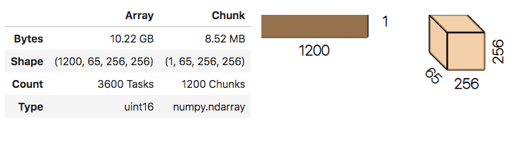
No data has been read from disk yet!
napari is capable of consuming Dask arrays,
so you can simply call napari.imshow on this stack and behind the scenes,
Dask will take care of reading the data from disk
and handing a numpy array to napari each time a new timepoint or channel is requested.
import napari

# specify contrast_limits and multiscale=False with big data
# to avoid unnecessary computations
napari.imshow(stack, contrast_limits=[0,2000], multiscale=False)
Note: providing the contrast_limits and multiscale arguments prevents napari from trying to calculate the data min/max, which can take an extremely long time with big data.
See napari issue #736 for further discussion.
Make your life easier with dask-image#
This pattern for creating a dask.array from image data
has been previously described in an excellent blog post by John Kirkham.
It is a common-enough pattern that John created a useful library (dask-image)
that does all this for you,
provided your image format can be read by the pims (Python Image Sequence) reader
(if not, see note above about providing your own reader function with dask.delayed).
Using dask-image, all of the above code can be simplified to 5 lines:
import napari
from dask_image.imread import imread

stack = imread("/path/to/experiment/*.tif")
napari.imshow(stack, contrast_limits=[0,2000], multiscale=False)
Side note regarding higher-dimensional datasets#
In the above example, it would be quite common to have a 5+ dimensional dataset
(e.g. different timepoints and channels represented among the 3D TIFF files in a folder).
A standard approach to deal with that sort of thing in numpy would be to reshape the array after instantiation.
With Dask, reshaping arrays can sometimes lead to unexpected read events if you’re not careful.
For example:
from dask_image.imread import imread
stack = imread('/path/to/experiment/*.tif')
stack.shape  # -> something like (1200, 64, 256, 280)
stack[0].compute()  # incurs a single file read

# if there were two channels in that folder you might try to do this:
stack = stack.reshape(2, 600, 64, 256, 280)
# but now trying to read just the first timepoint in the first channel:
stack[0, 0].compute()  # incurs 600 read events!
We will update this post as best-practices emerge,
but one possible solution to this is to avoid reshaping
Dask arrays altogether, by constructing multiple Dask arrays using dask-image, and then using
da.stack to combine them:
from dask_image.imread import imread
import dask.array as da

# # instead of this
# stack = imread('/path/to/experiment/*.tif')
# stack = stack.reshape(2, 600, 64, 256, 280)
# stack[0, 0].compute()  # incurs 600 read events!

# do something like this:
file_pattern = "/path/to/experiment/*ch{}*.tif"
channels = [imread(file_pattern.format(i)) for i in range(nchannels)]
stack = da.stack(channels)
stack.shape  # (2, 600, 64, 256, 280)
stack[0, 0].compute()  # incurs a single file read
A real example: high-resolution human brain imaging dataset#
In this example, we are going to view and process a high-resolution human brain imaging dataset. The dataset was obtained from Dr. Brian Edlow’s Lab for NeuroImaging of Coma and Consciousness, which is dedicated to promoting recovery of consciousness in people with severe brain injuries. This dataset is a 100 micron resolution magnetic resonance imaging (MRI) scan of an ex vivo human brain specimen. The brain specimen was donated by a 58-year-old woman who had no history of neurological disease and died of non-neurological causes. This dataset was originally described in Edlow, B.L., Mareyam, A., Horn, A. et al. 7 Tesla MRI of the ex vivo human brain at 100 micron resolution. Sci Data 6, 244 (2019).
Getting the data
You can download the dataset from here.
In this example we use the FLASH25_100um_TIFF_Axial data. This link will download a ~2 Gb .zip file and after extracting the compressed data set,
the .tiff images can be found in the SYNTHESIZED_TIFF_Images_Raw/Synthesized_FLASH25_100um_TIFF_Axial_Images/
directory. The dataset is 3.69 GB unzipped.
While we could use plain dask through delayed, as we have shown above, we
will make our lives easier here and use
dask-image.
Using dask_image.imread, loading the entire dataset to view in napari is straightforward.
import napari
from dask_image.imread import imread

# Load images
images = imread(
    'SYNTHESIZED_TIFF_Images_Raw/Synthesized_FLASH25_100um_TIFF_Axial_Images/Synthesized_FLASH25_Axial_*.tiff'
    )
napari.imshow(images)

if __name__ == '__main__':
    napari.run()
And here’s the final output!
Processing data with dask.array.map_blocks#
As previously mentioned, sometimes it is desirable to process data prior to viewing. We’ll take as an example a series of TIFF files acquired on a lattice-light-sheet microscope. A typical workflow might be to deskew, deconvolve, and perhaps crop or apply some channel registration prior to viewing.
With dask.array.map_blocks we can apply any function that accepts a numpy array
and returns a modified array to all the images in our dask.array.
It will be evaluated lazily, when requested (in this case, by napari);
we do not have to wait for it to process the entire dataset.
Here is an example of a script that will take a folder of raw tiff files,
and lazily read, deskew, deconvolve, crop,
and display them, on demand as you move the napari dimensions sliders around.
import napari
import pycudadecon
from functools import partial
from skimage import io
from dask_image.imread import imread

# load stacks with dask_image, and psf with skimage
stack = imread("/path/to/experiment/*.tif")
psf = io.imread("/path/to/psf.tif")

# prepare some functions that accept a numpy array
# and return a processed array

def last3dims(f):
    # this is just a wrapper because the pycudadecon function
    # expects ndims==3 but our blocks will have ndim==4
    def func(array):
        return f(array[0])[None, ...]
    return func


def crop(array):
    # simple cropping function
    return array[:, 2:, 10:-20, :500]

# https://docs.python.org/3.8/library/functools.html#functools.partial
deskew = last3dims(partial(pycudadecon.deskew_gpu, angle=31.5))
deconv = last3dims(partial(pycudadecon.decon, psf=psf, background=10))
# note: this is done in two steps just as an example...
# in reality pycudadecon.decon also has a deskew argument

# map and chain those functions across all dask blocks
deskewed = stack.map_blocks(deskew, dtype="uint16")
deconvolved = deskewed.map_blocks(deconv, dtype="float32")
cropped = deconvolved.map_blocks(crop, dtype="float32")

# put the resulting dask array into napari.
# (don't forget the contrast limits and multiscale==False !)
viewer, _ = napari.imshow(
    cropped,
    contrast_limits=[90, 1500],
    multiscale=False,
    ndisplay=3,
    scale=(3, 1, 1),
)

napari.run()
Of course, the GUI isn’t as responsive as it would be if you had processed the data up front
and loaded the results into RAM and viewed them in napari (it’s doing a lot of work after all!),
but it’s surprisingly usable,
and allows you to preview the result of a relatively complex processing pipeline on-the-fly,
for arbitrary timepoints/channels, while storing only the raw data on disk.
This workflow is very much patterned after another great post by John Kirkham, Matthew Rocklin, and Matthew McCormick
that describes a similar image processing pipeline using ITK.
napari simply sits at the end of this lazy processing chain,
ready to show you the result on demand!