Triangulation backends for the napari Shapes layer#
Background#
In order to draw polygons and polygon edges to the screen, napari first needs to break these shapes up into triangles, a fundamental graphical element understood by graphics frameworks like OpenGL. This process is called triangulation.
In the beginning, napari directly used a simple triangulation implementation provided by Vispy. Two issues with the Vispy implementation were that it was slow, and that it could not account for complicated shapes like polygons with holes in them.
Show code cell source
import numpy as np
import matplotlib.pyplot as plt
from vispy.geometry.triangulation import Triangulation
from triangle import triangulate
from bermuda import triangulate_polygons_face
from napari.layers.shapes._accelerated_triangulate_python import (
        normalize_vertices_and_edges_py
        )

def vispy_triangulate(vertices, edges):
    tri = Triangulation(np.copy(vertices), np.copy(edges))
    tri.triangulate()
    return tri.pts, tri.tris

# 0. Make data

# outline of South Africa
za = np.array(
    [[-28.58, 196.34], [-28.08, 196.82], [-28.36, 197.22], [-28.78, 197.39],
     [-28.86, 197.84], [-29.05, 198.46], [-28.97, 199.  ], [-28.46, 199.89],
     [-24.77, 199.9 ], [-24.92, 200.17], [-25.87, 200.76], [-26.48, 200.67],
     [-26.83, 200.89], [-26.73, 201.61], [-26.28, 202.11], [-25.98, 202.58],
     [-25.5 , 202.82], [-25.27, 203.31], [-25.39, 203.73], [-25.67, 204.21],
     [-25.72, 205.03], [-25.49, 205.66], [-25.17, 205.77], [-24.7 , 205.94],
     [-24.62, 206.49], [-24.24, 206.79], [-23.57, 207.12], [-22.83, 208.02],
     [-22.09, 209.43], [-22.1 , 209.84], [-22.27, 210.32], [-22.15, 210.66],
     [-22.25, 211.19], [-23.66, 211.67], [-24.37, 211.93], [-25.48, 211.75],
     [-25.84, 211.84], [-25.66, 211.33], [-25.73, 211.04], [-26.02, 210.95],
     [-26.4 , 210.68], [-26.74, 210.69], [-27.29, 211.28], [-27.18, 211.87],
     [-26.73, 212.07], [-26.74, 212.83], [-27.47, 212.58], [-28.3 , 212.46],
     [-28.75, 212.2 ], [-29.26, 211.52], [-29.4 , 211.33], [-29.91, 210.9 ],
     [-30.42, 210.62], [-31.14, 210.06], [-32.17, 208.93], [-32.77, 208.22],
     [-33.23, 207.46], [-33.61, 206.42], [-33.67, 205.91], [-33.94, 205.78],
     [-33.8 , 205.17], [-33.99, 204.68], [-33.79, 203.59], [-33.92, 202.99],
     [-33.86, 202.57], [-34.26, 201.54], [-34.42, 200.69], [-34.8 , 200.07],
     [-34.82, 199.62], [-34.46, 199.19], [-34.44, 198.86], [-34.  , 198.42],
     [-34.14, 198.38], [-33.87, 198.24], [-33.28, 198.25], [-32.61, 197.93],
     [-32.43, 198.25], [-31.66, 198.22], [-30.73, 197.57], [-29.88, 197.06],
     [-29.88, 197.06], [-28.58, 196.34], [-28.96, 208.98], [-28.65, 208.54],
     [-28.85, 208.07], [-29.24, 207.53], [-29.88, 207.  ], [-30.65, 207.75],
     [-30.55, 208.11], [-30.23, 208.29], [-30.07, 208.85], [-29.74, 209.02],
     [-29.26, 209.33], [-28.96, 208.98]],
     dtype=np.float32
    )

lat, lon = za.T

# 1. Get triangulation input data (vertices and edges)
vertices, edges = normalize_vertices_and_edges_py(za, close=True)

# 2. Compute triangulations
v_vispy, t_vispy = vispy_triangulate(vertices, edges)
tri_triangle = triangulate({'vertices': vertices, 'segments': edges}, opts='p')
v_triangle, t_triangle = tri_triangle['vertices'], tri_triangle['triangles']
t_bermuda, v_bermuda = triangulate_polygons_face([za])

# 3. Make the figure
fig, axes = plt.subplots(nrows=2, ncols=2)

axes[0, 0].fill(lon, lat)
axes[0, 0].set_title('polygon')

axes[0, 1].triplot(*v_vispy.T[[1, 0]], t_vispy)
axes[0, 1].set_title('vispy triangulation')

axes[1, 0].triplot(*v_triangle.T[[1, 0]], t_triangle)
axes[1, 0].set_title('triangle triangulation')

axes[1, 1].triplot(*v_bermuda.T[[1, 0]], t_bermuda)
axes[1, 1].set_title('bermuda triangulation')

fig.tight_layout()
fig.show()
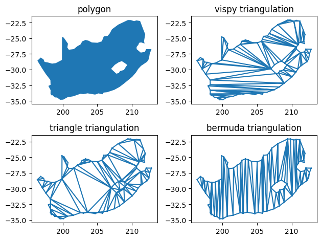
The issue of speed was partly resolved in napari 0.4.16 when Martin Weigert added the option to use triangle, a triangulation library written in C. However, triangle provided no error checking of input data, and some datasets could crash napari altogether. Also, triangle is distributed under a custom, non-standard license, which means that we are not allowed to distribute it with napari, and notably not in the bundled application.
Starting in napari 0.5.3, funded by a grant to the SpatialData project by CZI, PhD student Grzegorz Bokota started making dramatic improvements to napari’s triangulation capabilities, first by simplifying triangulation of simple shapes like circles and ellipses, then by reducing array allocations and implementing key operations in numba-accelerated functions, and finally by creating custom triangulation libraries in C++ (PartSegCore-compiled-backend) and Rust (bermuda). For complex shapes, these speedups added up to a 200-fold acceleration, all while improving robustness to malformed data. You can read more about this in our blog.
Usage#
So how do you take advantage of these speedups?
Install the backend you would like to use. By default, napari uses the pure Python backend, but you can also install numba (which will also accelerate the Labels layer, incidentally), triangle, PartSegCore-compiled-backend, or bermuda.
Open napari’s settings panel, then click on Experimental on the left hand navigation, and look for Triangulation backend.
Select “Fastest available” and napari will use the fastest installed backend. Otherwise, select a specific backend. napari will fall back on the Pure Python implementation if the backend is not installed. You might want to try different backends if a specific one is having issues with your data. If you do encounter issues, please let us know at napari/napari#issues.