Layers at a glance¶

Layers are the basic viewable objects that can be added to a viewer. napari supports seven main different layer types: Image, Labels, Points, Shapes, Surface, Tracks and Vectors. Each of the layer types corresponds to a different data type, visualization, and interactivity. You can add multiple layers of different types into the viewer and then start working with them, adjusting their properties.

All our layer types support n-dimensional data and the viewer provides the ability to quickly browse and visualize either 2D or 3D slices of the data.

After creating a napari.Viewer object, each layer for this object can be created by a corresponding viewer.add_<layer> method. For example, to add an Image layer named astronaut to the viewer object created from data, you can do

viewer = napari.Viewer()
viewer.add_image(data, name='astronaut')

To learn more about the layers available, see the Layers documentation. To learn about how to use the layers currently supported by napari, check out the Using layers how-to guides. For a gentle introduction, check out the Layer list section in the napari viewer tutorial.

Layer visibility¶

All our layers support a visibility toggle that allows you to set the visible property of each layer. This property is located inside the layer widget in the layers list and is represented by an eye icon.

Layer opacity¶

All our layers support an opacity slider and opacity property that allow you to adjust the layer opacity between 0, fully invisible and 1, fully visible.

Note

For the points layer, the opacity value applies globally to all the points in the layer, and so you don’t need to have any points selected for it to have an effect.
For the shapes layer, the opacity value applies individually to each shape in the layer, and so you must have shapes selected for it to have an effect.
For the vectors layer, the opacity value applies globally to all the vectors in the layer.
For the tracks layer, the opacity value applies globally to all the tracks in the layer.

Blending layers¶

All our layers support three blending modes: translucent, additive, and opaque. These modes determine how the visuals for this layer get mixed with the visuals from the other layers.

An opaque layer renders all the other layers below it invisible and will fade to black as you decrease its opacity.
A translucent setting will cause the layer to blend with the layers below it if you decrease its opacity but will fully block those layers if its opacity is 1. This is a reasonable default, useful for many applications.
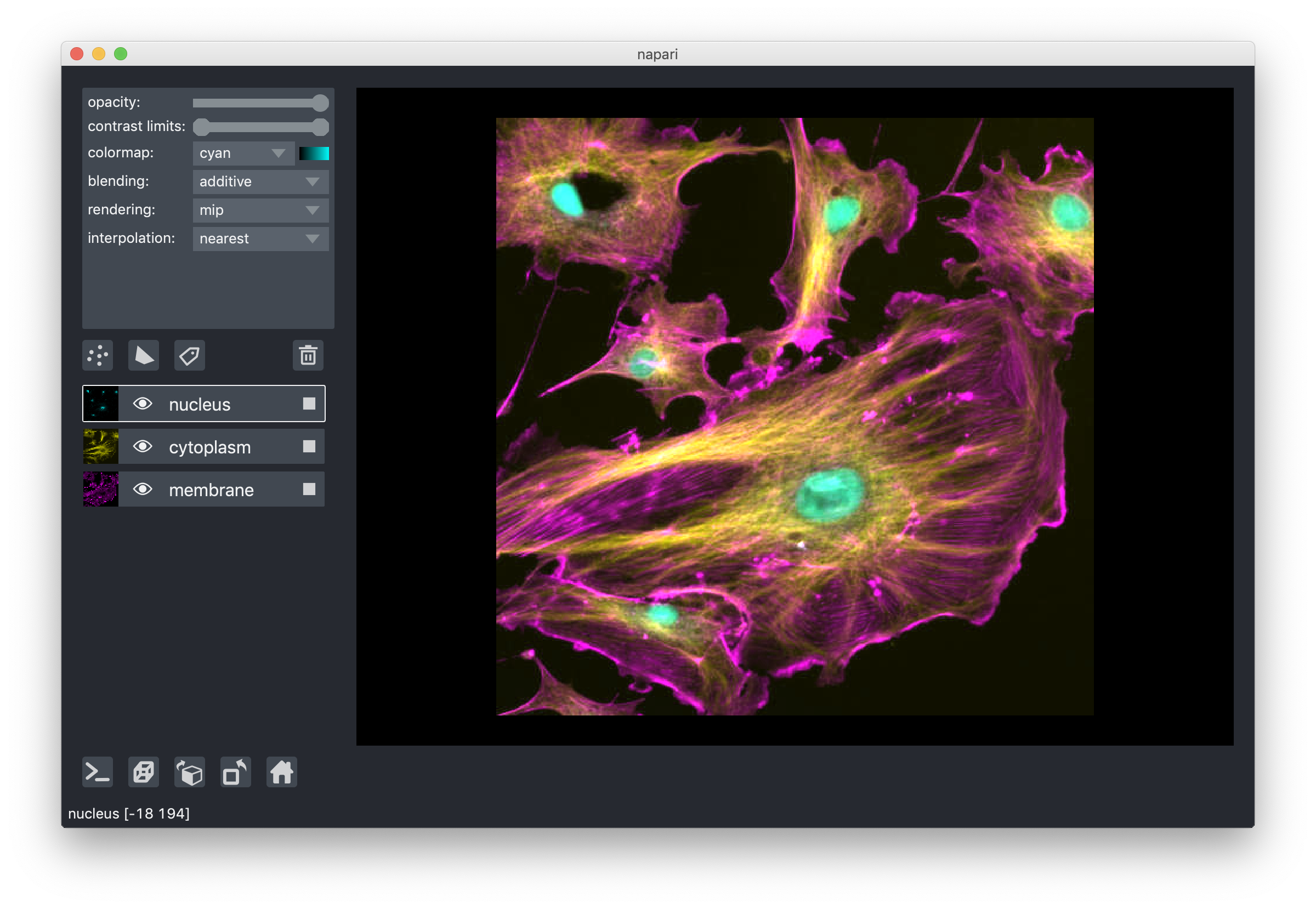
An additive blending mode will cause the layer to blend with the layers below even when it has full opacity. This mode is especially useful for visualizing multiple layers at the same time, such as cell biology applications where you have multiple different components of a cell labeled in different colors.

For example:

napari viewer with an image of a cell. Layer controls are open in the left sidebar with the blending set to additive.

3D rendering of images¶

All our layers can be rendered in both 2D and 3D mode, and one of our viewer buttons can toggle between each mode. The number of dimensions sliders will be 2 or 3 less than the total number of dimensions of the layer, allowing you to browse volumetric timeseries data and other high dimensional data. See for example these cells undergoing mitosis in this volumetric timeseries:

Note

Switching to 3D mode for a very large data set could trigger computation that leads to a memory error.

Layer interpolation¶

We support a variety of interpolation modes when viewing 2D slices. In the default mode nearest each pixel is represented as a small square of specified size. As you zoom in you will eventually see each pixel. In other modes neighbouring pixels are blended together according to different functions, for example bicubic, which can lead to smoother looking images. For most scientific use cases, nearest is recommended because it displays each data point, with no mixing of nearby data points. These modes have no effect when viewing 3D slices.

Layer rendering¶

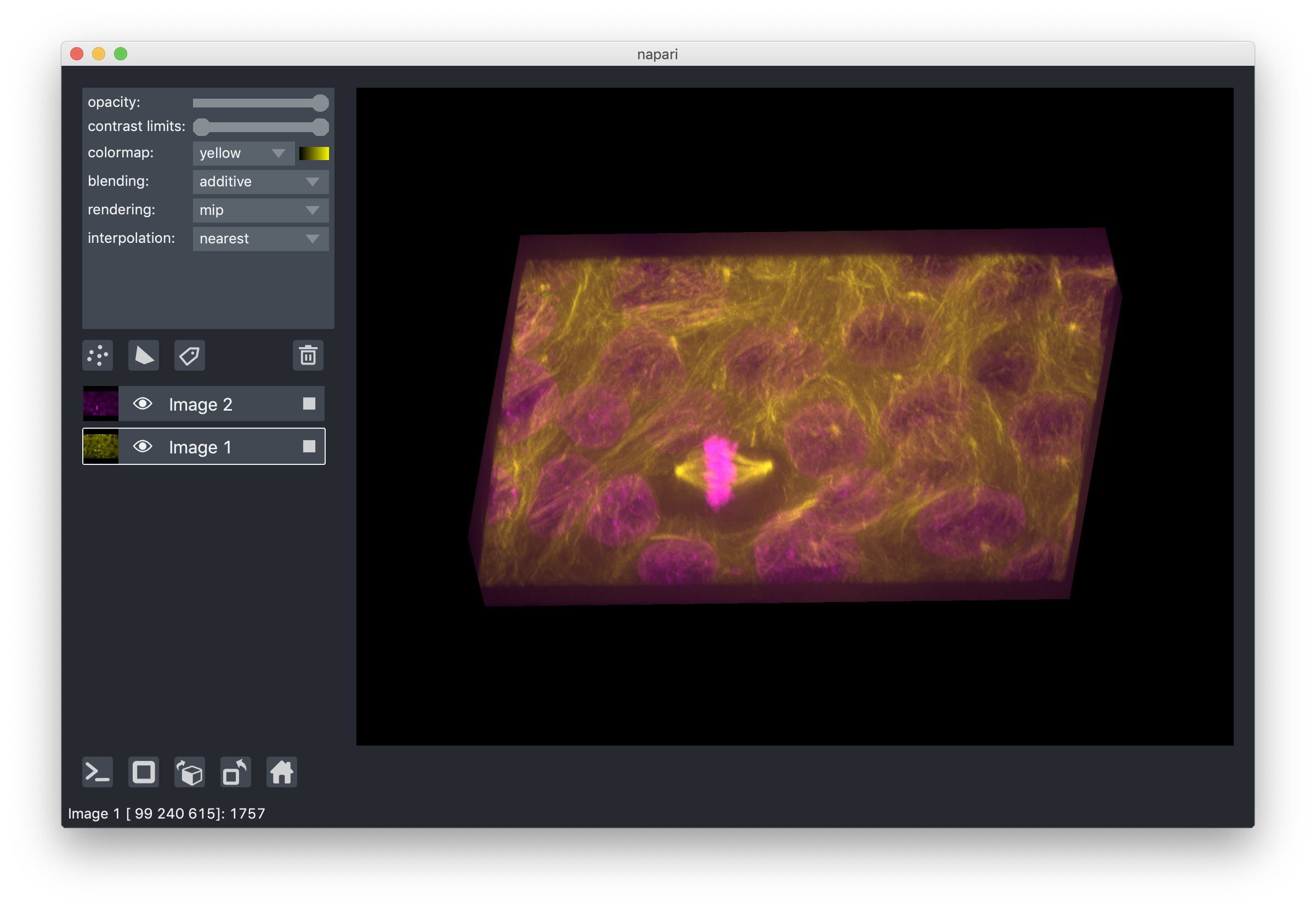
When viewing 3D slices, we support a variety of rendering modes. The default mode mip, or maximum intensity projection, will combine voxels at different distances from the camera according to a maximum intensity projection to create the 2D image that is then displayed on the screen. This mode works well for many biological images such as these cells growing in culture:

napari viewer with an image of cells in a culture. Layer controls are open in the left sidebar and rendering set to mip.

When viewing 2D slices the rendering mode has no effect.

Naming layers¶

All our layers support a name property that can be set inside a text box inside the layer widget in the layers list. The name of each layer is forced into being unique so that you can use the name to index into viewer.layers to retrieve the layer object.

Scaling layers¶

All our layers support a scale property and keyword argument that will rescale the layer multiplicatively according to the scale values (one for each dimension). This property can be particularly useful for viewing anisotropic volumes where the size of the voxel in the z dimension might be different then the size in the x and y dimensions.

In napari, you can scale the layers when creating an image layer or for an existing layer using the scale as a keyword argument or property respectively.

# scaling while creating the image layer
napari.view_image(retina, name='retina', scale=[1,10,1,1])
# scaling an existing layer
viewer.layers['retina'].scale = [1,10,1,1]

Translating layers¶

All our layers support a translate property and keyword argument that you can use to offset a layer relative to the other layers, which could be useful if you are trying to overlay two image tiles acquired with different stage positions.

Layer metadata¶

All our layers also support a metadata property and keyword argument that you can use to store an arbitrary metadata dictionary on the layer.

napari viewer tutorial

napari tutorials