napari viewer tutorial

Welcome to the tutorial on the napari viewer!

This tutorial assumes you have already installed napari and know how to launch the viewer. For help with installation see our installation tutorial. For help getting started with the viewer see our getting started tutorial.

This tutorial will teach you about the napari viewer, including how to use its graphical user interface (GUI) and how the data within it is organized. At the end of the tutorial you should understand the both the layout of the viewer on the screen and the data inside of it.

Launching the viewer

As discussed in getting started tutorial the napari viewer can be launched from the command-line, a python script, an IPython console, or a jupyter notebook. All four methods launch the same viewer, and anything related to the interacting with the viewer on the screen applies equally to all of them. We will use the syntax inside python scripts so you can copy and paste these examples into scripts and run them.

Let’s get stated by launching a viewer with a simple 2D image.

The fastest way to get the viewer open and throw an image up on the screen is using the napari.view_image method:

import napari
from skimage import data

viewer = napari.view_image(data.astronaut(), rgb=True)

Calling napari.view_image will return a Viewer object that is the main object inside napari. All the data you add to napari will be stored inside the Viewer object and will be accessible from it. This command will also open the viewer to create a GUI that you can interact with.

You can also create an empty Viewer directly and then start adding images to it. For example:

viewer = napari.Viewer()
new_layer = viewer.add_image(data.astronaut(), rgb=True)

add_image accepts the same arguments as view_image but returns a layer rather than a Viewer, (as you must already have a viewer to use it).

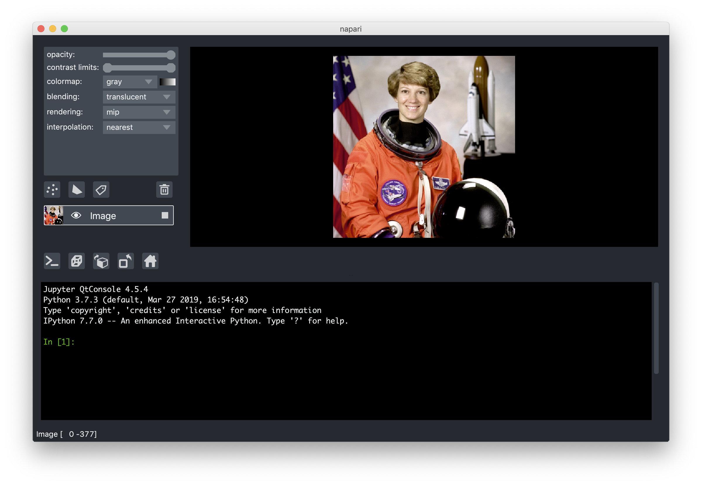
After running either of those two commands you should now be able to see the photograph of the astronaut in the napari viewer as shown below

from napari.utils import nbscreenshot

nbscreenshot(viewer)

Both the view_image and the add_image methods accept any numpy-array like object as an input, including n-dimensional arrays. For more information on adding images to the viewer see the image layer guide. Now we will continue exploring the rest of the viewer.

Layout of the viewer

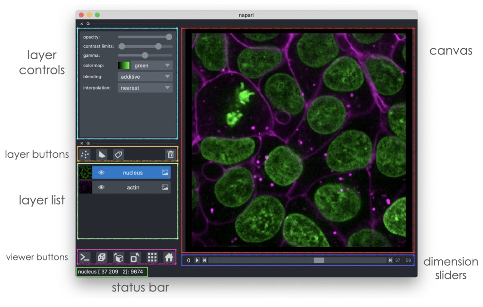
The viewer is organized into a few key areas:

We’ll go through each of these in the next sections.

Main canvas

The main canvas is in the center of the viewer and contains the visual display of the data passed to napari, including images, point, shapes, and our other supported data types. Under the hood the canvas is a vispy.scene.SceneCanvas object which has built-in support for features such as zooming and panning. As vispy uses OpenGL and your graphics card, panning and zooming are highly performant. You can also return to the original zoom level by clicking the home button in the viewer buttons panel.

Layer list

One of the basic napari objects are layers. There are different layer types for Image, Points, Shapes, and other basic data types. They can be added to the viewer either programmatically or through the GUI. Once added they start to populate the layer list located on the bottom lefthand side of the main canvas.

The layer list contains one widget for each of the layers that have been added to the viewer and includes a thumbnail which shows a miniaturized version of the currently viewed data, a name that is an editable text box, visibility button that can be toggled on or off to show or hide the layer, and an icon for the layer type.

Adding the following three image layers using the code below adds three-layer widgets to the layer list as follows:

viewer = napari.Viewer()
viewer.add_image(data.astronaut(), name='astronaut')
viewer.add_image(data.moon(), name='moon')
viewer.add_image(data.camera(), name='camera')

nbscreenshot(viewer)

Note that we’ve also also named each of the layers using the name keyword argument in add_image, and that name has appeared as a string in the layer widget. The layer name is coerced into being unique so that it can be used to index into the LayerList.

You can select layers, causing them to become outlined, by clicking on their layer widget. Multiple layers can be simultaneously selected using either shift or command click to select either all the layers in between clicked-on layers or just the clicked-on layers respectively.

You can rearrange the order of the layers by dragging them, including dragging multiple layers at the same time.

The Viewer object also contains our LayerList object that allows you to access the data of all the layers by

viewer.layers

[<Image layer 'astronaut' at 0x15050fe80>, <Image layer 'moon' at 0x15050f370>, <Image layer 'camera' at 0x15050f880>]

This object can be indexed like a normal list using an int or using the str name of the layer as follows

viewer.layers[0]

<Image layer 'astronaut' at 0x15050fe80>

viewer.layers['astronaut']

<Image layer 'astronaut' at 0x15050fe80>

You can rearrange layers by clicking and dragging them.

Layer controls

Above the layers list in the top left corner of the viewer there is a box that contains the layer controls. The controls that you have available to you depend on the layer type that you have selected.

For example, if you add a Points layer after adding an Image layer you will now see different controls present.

import numpy as np

viewer = napari.view_image(data.astronaut(), rgb=True)
points = np.array([[100, 100], [200, 200], [300, 100]])
viewer.add_points(points, size=30)

nbscreenshot(viewer)

Adjusting these properties in the GUI will cause corresponding changes to properties on the individual layers that are accessible in the console through viewer.layers.

For example, the name and opacity of a layer can be changed within the console as follows:

viewer.layers[0].name = 'astronaut'
viewer.layers[0].opacity = 0.7

and these changes will instantly propagate to the GUI. For more information about the different properties for different layer types please see our layer specific tutorials listed at the bottom of this tutorial.

New layer buttons

New Points, Shapes, and Labels layers can be added to the viewer using the new layer buttons in the bottom righthand corner of the GUI. These correspond to the calls such as:

viewer.add_points(data)
viewer.add_shapes(data)
viewer.add_labels(data)

but with empty data. Once added in the GUI these layers become accessible in the layers list and at viewer.layers.

Layers can also be deleted by selecting them and then clicking on the trash icon, or by dragging the layers and dropping them into the trash.

In the console a layer at index i can be removed by

viewer.layers.pop(i)

Dimension sliders

One of the main strengths of napari is that it has been designed from the beginning to handle n-dimensional data. While much consumer photography is 2D and RGB, scientific image data can often be volumetric (i.e. 3D), volumetric timeseries (i.e. 4D), or even higher dimensional. napari places no limits on the dimensionality of its input data for all its layer types.

Adding data with a dimensionality greater than 2D will cause dimension sliders to appear directly underneath the main canvas and above the status bar. As many sliders as needed will appear to ensure the data can be fully browsed. For example, a 3D dataset needs one slider, a 4D dataset needs two sliders, and so on. The widths of the scroll bars of the dimension sliders are directly related to how many slices are in each dimension.

It is also possible to mix data of different shapes and dimensionality in different layers. If a 2D and 4D dataset are both added to the viewer then the sliders will only affect the 4D dataset and the 2D dataset will be remain the same. Effectively, the two datasets are broadcast together using NumPy broadcasting rules.

For example, the following commands from the console will add a both 2D and 3D datasets to the same viewer:

viewer = napari.Viewer()
viewer.add_image(data.moon(), name='moon')
blobs = np.stack(
    [
        data.binary_blobs(
            length=512, blob_size_fraction=0.05, n_dim=2, volume_fraction=f
        )
        for f in np.linspace(0.05, 0.5, 10)
    ],
    axis=0,
).astype(float)
viewer.add_image(blobs, name='blobs', opacity=0.5, colormap='red')

nbscreenshot(viewer)

Viewer buttons

Underneath the layers list there is a row of buttons that includes the Console button that will show or hide our console that allows you to interact with a python kernel. Inside the console you can access the viewer using the viewer argument.

When the console button is clicked, the console will appear at the bottom of the viewer as follows:

We then have a button that switches between 2D and 3D rendering. After running the following code:

from scipy import ndimage as ndi

blobs = data.binary_blobs(length=128, volume_fraction=0.1, n_dim=3)
viewer = napari.view_image(blobs.astype(float), name='blobs')
labeled = ndi.label(blobs)[0]
viewer.add_labels(labeled, name='blob ID')

… clicking on the 3D button

and rotating the camera view with the mouse gives something like the following view:

# programmatically adjust the camera angle
viewer.dims.ndisplay = 3
viewer.camera.zoom = 2
viewer.camera.angles = (3, 38, 53)
nbscreenshot(viewer)

Next to the 2D / 3D button is a button to roll the dimensions that are currently being displayed in the viewer - for example if you have a ZYX volume and are looking at the YX slice this will then show you the ZY slice.

After that is a button that transposes the displayed dimensions.

Finally, there is the home button that will reset the camera state to its initial values.

Status bar

At the very bottom of the GUI there is a status bar that contains useful updates and tips.

On the lefthand side of the status bar there is a message that contains information about the position of the mouse and the values of any images or the indices of any points that are currently hovered over, depending on which layer is selected. The status bar will also display information about what button you are clicking in the layer control panel too.

The righthand side of the status bar contains some helpful tips depending on which layer and tools are currently selected.

Changing viewer theme

Currently, napari comes with two different themes light and dark, which is the default. To change the theme, update theme property of the viewer:

viewer = napari.Viewer()
viewer.add_image(data.astronaut(), name='astronaut')

# change the viewer theme
viewer.theme = 'light'

nbscreenshot(viewer)

Adding your own custom theme isn’t too hard either but does require creating your own color palette and rebuilding the icons. If people want more themes, we’re happy to add them or if you look at our contributing guidelines for more information about building the icons and add one yourself!

Custom keybinding

One of the promises of napari is to provide a beginner friendly environment for interactive analysis. For example, we want to enable workflows where people can interact with the GUI, say click on the centers of some objects, or paint over some regions and then perform custom analysis. As a first step towards enabling custom interactivity we’ve provided support to add your own custom keybindings to the Viewer or individual Layer objects such that when the corresponding key gets clicked your custom function gets executed. Depending on which object you bind your key to, your function will either get access to the state of the entire viewer or layer object.

For example, to bind function that loops through all layers in the viewer and prints their names to your console when you press the p key you can do the following:

viewer = napari.Viewer()
viewer.add_image(data.astronaut(), name='astronaut')

@viewer.bind_key('p')
def print_names(viewer):
    print([layer.name for layer in viewer.layers])

By default, your key will bind to the key press event, but it is also possible to bind to the key release event by including a yield inside your function. All code before the yield will get executed on key press and all code after the yield will get executed on key release. The following example will print hello when you start to press the m key and print goodbye when you release it.

viewer = napari.Viewer()
viewer.add_image(data.astronaut(), name='astronaut')

@viewer.bind_key('m')
def print_message(viewer):
    print('hello')
    yield
    print('goodbye')

viewer.close()

Keys can be bound both to the object class or a particular instance depending on if you want the keybinding to apply to all instances of the class or only one particular instance.

Currently the keybindings only work when the main canvas is in focus, we are working to ensure they always work.

The ability to add custom keybindings dramatically increases what is possible within napari and we hope you take full advantage of them.

Next steps

Hopefully, this tutorial has given you an overview of the functionality available on the napari viewer, including the LayerList and some of the different layer types. To learn more about the different layer types that napari supports, check out our guides on using layers.

previous

Getting started with napari

next

Layers at a glance